Introduction

A Risk-based optimal portfolio is the portfolio that, in some sense, has the best combination between the expected rate of return and the dispersion of possible outcomes.

Given a portfolio, we can estimate its expectation of return. The actual realization of an investment in this portfolio could be larger or smaller than this expectation. Therefore, the dispersion of possible outcomes around the expectation of return is vital information to an investor. A smaller dispersion value may translate to lower probability for outcomes far below the expected return.

The dispersion of possible outcomes is often called risk. The quantity that measures the dispersion of possible outcomes is called dispersion or risk measure. In this document we will use both terms interchangeably.

The dispersion measure can be defined in many ways. azapy package provides a comprehensive collection of risk-based portfolio optimization strategies based on the following dispersion measures:

• mCVaR - mixture Conditional Value at Risk,

• mSMCR - mixture Second Moment Coherent Risk,

• mMAD - m-level Mean Absolute Deviation,

• mLSD - m-level Lower Semi-Deviation,

• mBTAD - mixture Below Threshold Absolute Deviation,

• mBTSD - mixture Below Threshold Semi-Deviation,

• mEVaR - mixture Entropic Value at Risk

• GINI - Gini index,

• SD - Standard Deviation,

• VAR - Variance, leading to mean-variance, MV, type of models.

In each case several optimization strategies are implemented. To understand them better, let’s look at a generic example of portfolio frontiers graphically represented in the figure below.

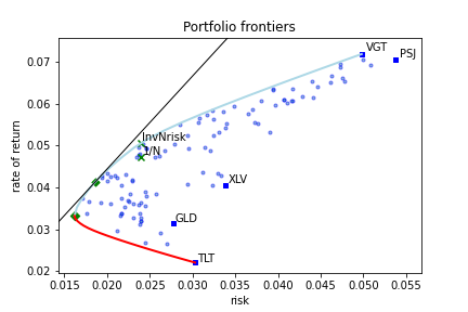
Fig 1. : Example of portfolio frontiers - risk vs. expected rate of return.

This is a typical representation of portfolio frontiers. On the x-axis we have the values of the dispersion measure (risk) while on the y-axis is the expected rate of returns. Several features are worth mentioning.

The blue line is called the efficient frontier. It represents the set of portfolios with the highest expected rate of returns for a given value of risk. These are the portfolios of interest for an investor.

The lower red line is called the inefficient frontier. These are the portfolios with the lowest rate of return for a given value of risk. Clearly, this family of portfolios is to be avoided by an investor.

The leftmost point, where the blue and red lines meet, is the Minimum Risk Portfolio (also called Global Minimum Risk Portfolio). This is the portfolio with the minimum risk among all possible portfolios. Investing in the minimum risk portfolio is a relative common strategy among professional investors.

The black straight line, in the upper part of the plot, is tangent to the efficient frontier. Its intersection with the y-axis (not shown in the plot) is at a level equal with the risk-free rate accessible to the investor. In this example the risk-free rate was set to 0. The point of tangency along the efficient frontier (in our plot depicted by a green diamond) is the tangency portfolio or the market portfolio. This is the portfolio that maximizes the \(\rho\)-Sharpe ratio. The \(\rho\)-Sharpe ratio[1] is defined as

\[\begin{equation*} \gamma = \frac{R - r_f}{\rho}, \end{equation*}\]

where:

• \(R\) is the portfolio expected rate of return,

• \(r_f\) is the risk-free rate accessible to the investor,

• \(\rho\) is the dispersion of portfolio rate of return.

Therefore, the portfolio that maximizes the \(\rho\)-Sharpe ratio is the portfolio with the highest expected excess rate of return (above the risk-free rate) per unit of risk, \(\rho\). This is a remarkable efficient portfolio often preferred by the investors.

All the points between the efficient (blue line) and inefficient (red line) frontiers are called inefficient portfolios.
There are no valid portfolios outside the portfolio frontiers.

The solid blue squares are the portfolios where the entire capital is allocated to a single component. They are labeled by the market symbol of this portfolio component. For short, we call them single asset portfolios.

Among the inefficient portfolios there is a remarkable one. That is the equal weighted portfolio. As the name suggested, all weights are equal to \(1/N\), where \(N\) is the number of portfolio components. Hence, its name \(1/N\)-portfolio or inverse-N portfolio. In our plot this portfolio is represented by a green x with label \(1/N\).

On the efficient frontier, we have its correspondent. In our plot it is depicted by a green x with label InvNrisk. This is the efficient portfolio that has the same risk as the equal weighted portfolio. In-sample both portfolios have the same risk while the expected rate of returns is larger for InvNrisk than for inverse-N portfolio. However, out-of-sample, especially for a short period of observations, equal weighted may outperform InvNrisk portfolio.

Another way to visualize the portfolio frontiers is presented in the following figure.

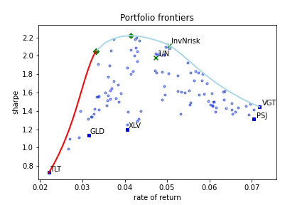
Fig 2. : Example of portfolio frontiers - expected rate of return vs. Sharpe ratio.

It contains the same information as Fig. 1. However, now on the x-axis is the expected rate of return while on the y-axis is the \(\rho\)-Sharpe ratio. We have preserved the color code and all the symbols from Fig. 1.

Fig. 2. gives a better understanding of portfolio efficiency in terms of expected excess return per unit or risk.

For all dispersion measures mentioned above, the azapy package offers the following portfolio optimization strategies:

1. Minimization of risk for targeted expected rate of return. This is the most common portfolio optimization strategy. It returns portfolios along the efficient frontier (blue line in Figs. 1 and 2). The strategy requires the user to input the desired value of the expected rate of return. This value must be between the expected rate of return of minimum risk portfolio and the highest expected rate of return among the portfolio components. If the input value is outside of this range then it will automatically default to the nearby limit. In our implementation this strategy is designated by setting rtype='Risk'.

2. Minimum risk portfolio. This is the efficient portfolio with minimum risk (the most left limit of the efficient frontier). It is a common strategy among professional investors. It is available under the setting rtype='MinRisk'.

3. Maximization of expected rate of return for targeted risk value. The strategy returns portfolios along the efficient frontier (blue line in Fig. 1 and 2). Requires the user to enter the desired value of risk. In general, it is not intuitive for an investor to specify outright a rational value for risk. However, this strategy is useful if we want to find an efficient portfolio that has the same risk as a benchmark portfolio. The most common example is the efficient portfolio with the same risk as the equal weighted portfolio. In our implementation this strategy is designated by setting rtype='InvNrisk'. It allowed to enter any benchmark portfolio by specifying the weights (long only, i.e., non-negative weights).

4. Maximization of the expected rate of return for fixed risk-aversion factor. In this strategy the optimal portfolio weights maximize the quantity \(R -\lambda \rho\), where \(R\) is the portfolio expected rate of returns, \(\rho\) is the risk, and \(\lambda\) is the risk-aversion factor. \(\lambda\) takes values between \(0\) and \(+\infty\). For \(\lambda=0\) the optimal portfolio is the single asset portfolio where the entire capital is allocated to the component with the highest expected rate of return. This is the rightmost point along the efficient frontier. For \(\lambda=+\infty\) the optimal portfolio is the minimum risk portfolio, the leftmost point on the efficient frontier. Any other values for \(\lambda\) will lead to an optimal portfolio along the efficient frontier. In general, it is not intuitive for an investor to specify a rational value for the risk-aversion factor. Note that the same value of \(\lambda\) may lead to different portfolio compositions for different dispersion measures and market conditions. Therefore, a direct use of
   this strategy, by specifying a desired value for \(\lambda\), may not be convenient. However, this strategy may be useful if it is combined with a strategy to estimate the value of risk-aversion factor based on market conditions (e.g., technical analysis, etc.). In our implementation this optimization strategy is designated by setting rtype='RiskAverse'.

5. Maximization of \(\rho\)-Sharpe ratio. This is the portfolio with the highest expected excess rate of return per unit of risk held by the investor. It is a very popular strategy among investors. In our implementation this strategy is designated by setting rtype='Sharpe'.

6. Minimization of inverse \(\rho\)-Sharpe ratio. Obviously, this strategy is logically equivalent with the one above. It returns the same portfolio weights. However, from a numerical point of view, the minimization of inverse Sharpe ratio and the maximization of Sharpe ratio have quite different implementations. Both implementations have similar accuracy and computational speed. For completeness, we chose to make available this implementation under the setting rtype='Sharpe2'.

azapy package covers, 9 risk-based dispersion measures \(\times\) 6 optimization strategies, in total 54 risk-based portfolio optimization strategies.[2]

The rigorous mathematical description of these strategies is presented here.

The natural question that arises is: which one is the best?

There is no absolute answer to this question and so there is no substitute for our personal research. To this end, azapy package provides the necessary analytical tools to perform a comprehensive quantitative portfolio analysis.

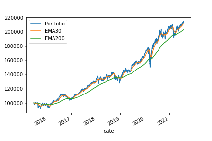
Fig 3. Example of out-of-sample (backtesting) portfolio performance.

An out-of-sample analysis, also called backtesting or historical simulation, can be performed for any of the implemented portfolio strategies. The following information can be extracted:

1. Portfolio realized rate of return. It is available monthly, annually and by rolling period. From these reports one can easily gauge the magnitude and seasonality of returns.

2. The realized drawdown events. It is a very important information that can give a measure (although limited to previous market events) for the amount and duration of losses that an investor may be exposed to.

3. Easy graphical and numerical comparisons between different strategies or different portfolios altogether.

Examples of how to carry out a portfolio out-of-sample analysis are present in a collection of Jupyter Notebooks and Python scripts. They can be used as a source of inspiration for further research.

Once we have decided for a portfolio composition and optimization strategy, azapy can help with portfolio maintenance. It can prove comprehensive information regarding the prevailing portfolio weights, number of shares, delta positions and cash flow at rebalancing time. An example is provided in a Jupyter Notebook.

azapy package has its own facility to collect historical market data from various providers[3] (see section Read historical market data).

---

[1]

The concept of Sharpe ratio was introduced in 1966 by William F. Sharpe. In the original definition \(\rho\) is the portfolio volatility \(\sigma\) (standard deviation). In our presentation we use a generalization of Sharpe ratio where the volatility is replaced by the prevailing dispersion measure, \(\rho\). We call it \(\rho\)-Sharpe.

[2]

Not all strategies are independent. For example, 'Sharpe' and 'Sharpe2' produce identical result (up to numerical precision) although, they have different numerical implementations. Also there are overlaps between MV and SD based strategies, etc..

[3]

Some of the market data providers require a valid API key.